How Effective is Bollinger Bands in KLSE?

Trading with Bollinger Bands

Bollinger Bands is a common strategy used by traders
I like the mathematical nature of this strategy,
using a smooth moving average line, and make a “band”
of n standard deviations (usually 2) away from the line.

This kinds of remind me of the mathematics of normal distribution curve.
I am not covering the mathematics behind this

I believe there is many more guides who can do better than me.
So in this article I will test the performance of Bollinger Bands on KLSE index.

Though we can’t directly buy the KLSE index,
we can achieve similar by buying futures or warrants that tracks the KLSE index.

Reading Data

I downloaded historical data of KLSE from Yahoo Finance in csv form.

We need to read it into memory to perform backtesting.

import pandas as pd

KLSE = pd.read_csv('KLSE.csv')
KLSE = KLSE.replace(',','', regex=True)
KLSE['Open'] = KLSE['Open'].astype(float)
KLSE['Close'] = KLSE['Close'].astype(float)
KLSE['Change'] = (KLSE['Close'] - KLSE['Close'].shift(1))/KLSE['Open'] + 1

KLSE.head()

	Date	Open	High	Low	Close	Adj Close	Volume	Change
0	4-Jan-10	1272.31	1275.75	1272.25	1275.75	1275.75	56508200	NaN
1	5-Jan-10	1278.26	1290.55	1278.26	1288.24	1288.24	136646600	1.009771
2	6-Jan-10	1288.86	1296.44	1288.02	1293.17	1293.17	117740300	1.003825
3	7-Jan-10	1293.69	1299.70	1290.36	1291.42	1291.42	115024400	0.998647
4	8-Jan-10	1294.93	1295.51	1290.86	1292.98	1292.98	74587200	1.001205

Rules

We are building a very simple strategy based on Bollinger Bands,
keep in mind that we are only using long strategy,
since shorting is usually harder in Malaysian market due to several factors.

the rules are:

When the daily close price moves above “Upper Boundary”, buy in.
When the daily close price moves below “Lower Boundary”, we sell our position (not shorting).
When the daily close price moves between “Upper Boundary” and “Lower Boundary”, hold previous position.
No trading cost.

def simulate(df,n):
    
    import talib
    
    df['UpperBand'], df['MiddleBand'],df['LowerBand'] = talib.BBANDS(df['Close'], timeperiod=n, nbdevup=2, nbdevdn=2, matype=0)
    
    df.dropna(inplace = True)

    gold_cross = df[df['Close'] > df['UpperBand']].index
    df.loc[gold_cross,'Cross'] = 1

    gold_cross = df[df['Close'] < df['LowerBand']].index
    df.loc[gold_cross,'Cross'] = 0
    
    df['Cross'].ffill(inplace=True)

    df['Buy'] = df['Cross'].diff()

    df['Return'] = df['Cross']*df['Change']

    def norm(x):
        if x == 0:
            return 1
        else:
            return x

    df['Return'] = df['Return'].apply(lambda x: norm(x))
    df['Nav'] = (df['Return']).cumprod()
    
    df.dropna(inplace=True)

    price_in = df.loc[df['Buy'] == 1,'Close'].values
    price_out = df.loc[df['Buy'] == -1,'Close'].values

    # divide by 252 because generally a year has 252 trading days
    num_periods = df.shape[0]/252
    rety = ((df['Nav'].iloc[-1] / df['Nav'].iloc[0]) ** (1 / (num_periods - 1)) - 1)*100.0

    if len(price_out) > len(price_in):
        price_out = price_out[:len(price_in)]
    
    if len(price_in) > len(price_out):
        price_in = price_in[:len(price_out)]
        
    VictoryRatio = ((price_out - price_in)>0).mean()*100.0
    DD = 1 - df['Nav']/df['Nav'].cummax()
    MDD = max(DD)*100.0

    return df, round(rety, 2), round(VictoryRatio, 2), round(MDD,2)

How Does This Strategy Works?

For easy explanation, see figure below

Green arrow indicates that daily close price had exceeded “Upper Boundary”, we buy in and hold

Red arrow indicates that daily close price had dropped below “Lower Boundary”, we sell our position

Demo,_,_,_ = simulate(KLSE.copy(),20)

import matplotlib.pyplot as plt
plt.style.use('seaborn')

# Take a portion of the dataset to visualize, 
# Otherwise the plot will be too small
Demo = Demo[500:1000]

ax = Demo['UpperBand'].plot(figsize=(10, 6),alpha=0.7)
Demo['Close'].plot(ax=ax,color='navy')
Demo['LowerBand'].plot(ax=ax,alpha=0.7)


# Buy signal
for p in Demo[Demo['Buy'] == 1].index:
    ax.plot(p,Demo['Close'][p],marker='^',color='green',markersize=15)

# Sell signal
for p in Demo[Demo['Buy'] == -1].index:
    ax.plot(p,Demo['Close'][p],marker='v',color='red',markersize=15)

plt.show()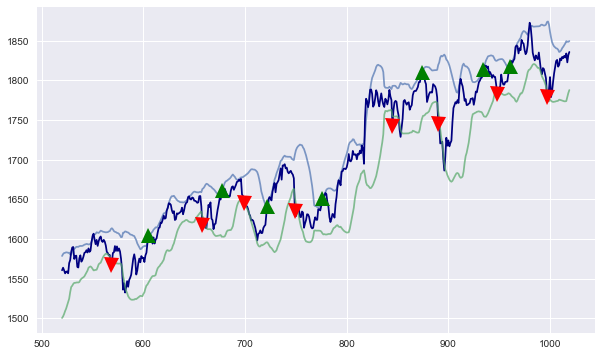

Strategy Performance

We are backtesting 3 values for Bollinger Band setting, 10,20,50

10 (Short term trade)
20 (Medium term trade)
50 (Medium-Long term trade)

BBandShort,cagrShort,vrShort,mddShort = simulate(KLSE.copy(),10)
BBandMed,cagrMed,vrMed,mddMed = simulate(KLSE.copy(),20)
BBandLong,cagrLong,vrLong,mddLong = simulate(KLSE.copy(),50)


KLSE['KLSE'] = (KLSE['Change']).cumprod()


ax = BBandShort.plot(x='Date',y='Nav',figsize=(10, 6))
BBandMed['Nav'].plot(ax=ax)
BBandLong['Nav'].plot(ax=ax)
KLSE['KLSE'].plot(ax=ax)
ax.legend(['n= 10','n = 20','n = 50','KLSE (benchmark)']);
ax.set_title('Growth of RM1 Invested')
plt.show()


from prettytable import PrettyTable

t = PrettyTable(['Strategy', 'CAGR', 'Win Rate', 'Max Drawdown'])
t.add_row(['Boll (10)', cagrShort,vrShort,mddShort])
t.add_row(['Boll (20)', cagrMed,vrMed,mddMed])
t.add_row(['Boll (50)', cagrLong,vrLong,mddLong])

print(t)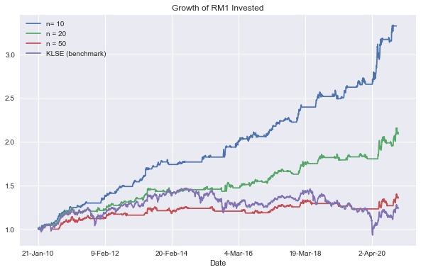

+-----------+-------+----------+--------------+
|  Strategy |  CAGR | Win Rate | Max Drawdown |
+-----------+-------+----------+--------------+
| Boll (10) | 13.19 |   50.0   |     5.57     |
| Boll (20) |  7.94 |  46.88   |     5.57     |
| Boll (50) |  3.3  |  35.71   |     7.91     |
+-----------+-------+----------+--------------+

Thoughts

From the results, it seems that the win rate is pretty bad, with 50% win rate as the best

However, this strategy seems to let traders avoid downturn and participate in upside moves.

The longer days setting for Bollinger Bands seem to perform the worst,
this might indicate that this strategy is suitable for short term trades only.

If you know coding,
you can try this out on other stocks that you like by getting csv data from Yahoo Finance.

This isn’t any trading advice and the studies and analysis done were for educational and sharing purposes only