Every successful trader is disciplined,
this is a quote that trader/investor had heard for too many times.
Every successful trade should have a plan to enter, plan to exit and cut loss, cut loss is a risk management technique,
it can theoretically prevent your losses from getting worse.
Today we are going to see if cut loss is a good strategy to protect your trade.
Common cut loss values are 5%, 10%,
but it is highly dependent on you risk preference,
there is no magic number for cut loss value, for this study we are using 5% cut loss value.
Reading Data
I downloaded historical data of KLSE from Yahoo Finance in csv form.
We need to read it into memory to perform backtesting.
import pandas as pd

KLSE = pd.read_csv('KLSE.csv')
KLSE = KLSE.replace(',','', regex=True)
KLSE['Open'] = KLSE['Open'].astype(float)
KLSE['Close'] = KLSE['Close'].astype(float)
KLSE['Change'] = (KLSE['Close'] - KLSE['Close'].shift(1))/KLSE['Open'] + 1

KLSE.head()| Date | Open | High | Low | Close | Adj Close | Volume | Change | |
|---|---|---|---|---|---|---|---|---|
| 0 | 4-Jan-10 | 1272.31 | 1275.75 | 1272.25 | 1275.75 | 1275.75 | 56508200 | NaN |
| 1 | 5-Jan-10 | 1278.26 | 1290.55 | 1278.26 | 1288.24 | 1288.24 | 136646600 | 1.009771 |
| 2 | 6-Jan-10 | 1288.86 | 1296.44 | 1288.02 | 1293.17 | 1293.17 | 117740300 | 1.003825 |
| 3 | 7-Jan-10 | 1293.69 | 1299.70 | 1290.36 | 1291.42 | 1291.42 | 115024400 | 0.998647 |
| 4 | 8-Jan-10 | 1294.93 | 1295.51 | 1290.86 | 1292.98 | 1292.98 | 74587200 | 1.001205 |
Rules
We are using very simple moving average + 5% stop loss as our strategy,
the rules are:
- when the “fast” moving average goes above the “slow” moving average, we buy in.
- when the “fast” moving average goes below the “fast” moving average, we sell.
- Cut loss when paper loss > 5%.
- No trading cost.
def simulate(df,fast,slow,cutloss = False):

    import talib

    df['fast'] = talib.SMA(df['Close'],fast)
    df['slow'] = talib.SMA(df['Close'],slow)

    df.dropna(inplace = True)

    gold_cross = df[df['fast'] > df['slow']].index
    df.loc[gold_cross,'Cross'] = 1

    gold_cross = df[df['fast'] < df['slow']].index
    df.loc[gold_cross,'Cross'] = 0

    df['Buy'] = df['Cross'].diff()

    df['Return'] = df['Cross']*df['Change']

    def norm(x):
        if x == 0:
            return 1
        else:
            return x

    df['Return'] = df['Return'].apply(lambda x: norm(x))
    df['Nav'] = (df['Return']).cumprod()

    DD = 1 - df['Nav']/df['Nav'].cummax()

    #===================================
    if cutloss:
        # set cutloss to 5.5% for extra buffer
        c = DD[DD > 0.055].index
        df.loc[c,'Cross'] = 0

        df['Buy'] = df['Cross'].diff()

        df['Return'] = df['Cross']*df['Change']

        df['Return'] = df['Return'].apply(lambda x: norm(x))
        df['Nav'] = (df['Return']).cumprod()

    #====================================

    # divide by 252 because generally a year has 252 trading days
    num_periods = df.shape[0]/252
    rety = ((df['Nav'].iloc[-1] / df['Nav'].iloc[0]) ** (1 / (num_periods - 1)) - 1)*100.0

    price_in = df.loc[df['Buy'] == 1,'Close'].values
    price_out = df.loc[df['Buy'] == -1,'Close'].values

    if len(price_out) > len(price_in):
        price_out = price_out[:len(price_in)]

    if len(price_in) > len(price_out):
        price_in = price_in[:len(price_out)]

    VictoryRatio = ((price_out - price_in)>0).mean()*100.0
    DD = 1 - df['Nav']/df['Nav'].cummax()
    MDD = max(DD)*100.0

    return df, round(rety, 2), round(VictoryRatio, 2), round(MDD,2)
Strategy Performance
We are backtesting 4 combinations
- 10 and 20 (Short term trade), No cut loss
- 20 and 50 (Medium term trade), No cut loss
- 10 and 20 (Short term trade), 5% cut loss
- 20 and 50 (Medium term trade), 5% cut loss
MA1020,cagr1020,vr1020,mdd1020 = simulate(KLSE.copy(),10,20,False)
MA2050,cagr2050,vr2050,mdd2050 = simulate(KLSE.copy(),20,50,False)
MA1020_cutloss,cagr1020_cutloss,vr1020_cutloss,mdd1020_cutloss = simulate(KLSE.copy(),10,20,True)
MA2050_cutloss,cagr2050_cutloss,vr2050_cutloss,mdd2050_cutloss = simulate(KLSE.copy(),20,50,True)

KLSE['KLSE'] = (KLSE['Change']).cumprod()
import matplotlib.pyplot as plt
plt.style.use('seaborn')

ax = MA1020['Nav'].plot(figsize=(10, 6))
MA2050['Nav'].plot(ax=ax)
MA1020_cutloss['Nav'].plot(ax=ax)
MA2050_cutloss['Nav'].plot(ax=ax)

KLSE['KLSE'].plot(ax=ax)
# plt.plot( 'Date','Nav', data = MA2050, marker='', color='olive', linewidth=2)
ax.legend(['MA1020','MA2050','MA1020 5% Cutloss','MA2050 5% Cutloss','KLSE']);
plt.show()


from prettytable import PrettyTable

t = PrettyTable(['Strategy', 'CAGR', 'Win Rate', 'Max Drawdown'])
t.add_row(['MA1020', cagr1020,vr1020,mdd1020])
t.add_row(['MA2050', cagr2050,vr2050,mdd2050])
t.add_row(['MA1020 5% Cutloss', cagr1020_cutloss,vr1020_cutloss,mdd1020_cutloss])
t.add_row(['MA2050 5% Cutloss', cagr2050_cutloss,vr2050_cutloss,mdd2050_cutloss])

print(t)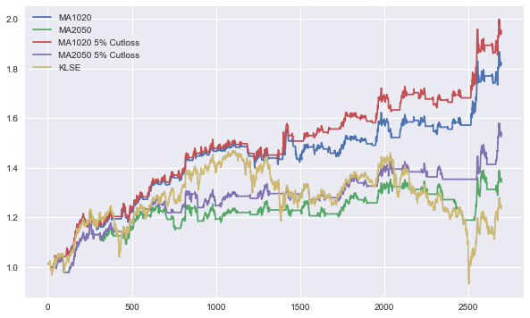
+-------------------+------+----------+--------------+
|      Strategy     | CAGR | Win Rate | Max Drawdown |
+-------------------+------+----------+--------------+
|       MA1020      | 6.44 |  50.77   |     8.52     |
|       MA2050      | 3.14 |  30.77   |    12.15     |
| MA1020 5% Cutloss | 7.19 |  45.21   |     5.44     |
| MA2050 5% Cutloss | 4.54 |  20.59   |     5.46     |
+-------------------+------+----------+--------------+
Thoughts
From the backtesting results,
cut loss seems to be a very effective risk management technique.
With 5% cut loss, it performed better than the same strategy without cut loss.
Although the win rate is lower,
this could mean that having cut loss,
you will realize your lossing trade more frequently
which is good as it prevents the trade from going south further.
If you know coding,
you can try this out on other stocks that you like by getting csv data from Yahoo Finance.
This isn’t any trading advice and the studies and analysis done were for educational and sharing purposes only