How Effective is Moving Average Strategy in KLSE?

Moving Average Strategy

Moving average strategy is a common strategy used by traders.

Unlike some of the more exotic indicators,
moving average readily available in many charting software or website such as klsescreener or tradingview

One common usage of moving average is that,
when the “fast” moving average goes above the “slow” moving average,
we buy in,
when the “fast” moving average goes below the “fast” moving average,
we sell.

So in this article I will test the performance of this strategy on KLSE index.

Though we can’t directly buy the KLSE index,
we can achieve similar by buying futures or warrants that tracks the KLSE index.

Reading data

I downloaded historical data of KLSE from Yahoo Finance in csv form.

We need to read it into memory to perform backtesting.

import pandas as pd

KLSE = pd.read_csv('KLSE.csv')
KLSE = KLSE.replace(',','', regex=True)
KLSE['Open'] = KLSE['Open'].astype(float)
KLSE['Close'] = KLSE['Close'].astype(float)
KLSE['Change'] = (KLSE['Close'] - KLSE['Close'].shift(1))/KLSE['Open'] + 1

KLSE.head()

	Date	Open	High	Low	Close	Adj Close	Volume
0	4-Jan-10	1272.31	1275.75	1272.25	1275.75	1275.75	56508200
1	5-Jan-10	1278.26	1290.55	1278.26	1288.24	1288.24	136646600
2	6-Jan-10	1288.86	1296.44	1288.02	1293.17	1293.17	117740300
3	7-Jan-10	1293.69	1299.70	1290.36	1291.42	1291.42	115024400
4	8-Jan-10	1294.93	1295.51	1290.86	1292.98	1292.98	74587200

Rules

We are using very simple moving average strategy,

the rules are:

1. when the “fast” moving average goes above the “slow” moving average, we buy in.
2. when the “fast” moving average goes below the “fast” moving average, we sell.
3. No trading cost.

def simulate(df,fast,slow):
    
    import talib

    df['fast'] = talib.SMA(df['Close'],fast)
    df['slow'] = talib.SMA(df['Close'],slow)
    
    df.dropna(inplace = True)

    gold_cross = df[df['fast'] > df['slow']].index
    df.loc[gold_cross,'Cross'] = 1

    gold_cross = df[df['fast'] < df['slow']].index
    df.loc[gold_cross,'Cross'] = 0

    df['Buy'] = df['Cross'].diff()

    df['Return'] = df['Cross']*df['Change']

    def norm(x):
        if x == 0:
            return 1
        else:
            return x

    df['Return'] = df['Return'].apply(lambda x: norm(x))
    df['Nav'] = (df['Return']).cumprod()

    price_in = df.loc[df['Buy'] == 1,'Close'].values
    price_out = df.loc[df['Buy'] == -1,'Close'].values

    # divide by 252 because generally a year has 252 trading days
    num_periods = df.shape[0]/252
    rety = ((df['Nav'].iloc[-1] / df['Nav'].iloc[0]) ** (1 / (num_periods - 1)) - 1)*100.0

    if len(price_out) > len(price_in):
        price_out = price_out[:len(price_in)]
    
    if len(price_in) > len(price_out):
        price_in = price_in[:len(price_out)]
        
    VictoryRatio = ((price_out - price_in)>0).mean()*100.0
    DD = 1 - df['Nav']/df['Nav'].cummax()
    MDD = max(DD)*100.0

    return df, round(rety, 2), round(VictoryRatio, 2), round(MDD,2)

Strategy Performance

We are backtesting 3 pairs of moving average

1. 10 and 20 (Short term trade)
2. 20 and 50 (Medium term trade)
3. 50 and 200 (Long term trade)

MA1020,cagr1020,vr1020,mdd1020 = simulate(KLSE.copy(),10,20)
MA2050,cagr2050,vr2050,mdd2050 = simulate(KLSE.copy(),20,50)
MA50200,cagr50200,vr50200,mdd50200 = simulate(KLSE.copy(),50,200)

KLSE['KLSE'] = (KLSE['Change']).cumprod()
import matplotlib.pyplot as plt
plt.style.use('seaborn')

ax = MA1020['Nav'].plot(figsize=(10, 6))
MA2050['Nav'].plot(ax=ax)
MA50200['Nav'].plot(ax=ax)
KLSE['KLSE'].plot(ax=ax)
# plt.plot( 'Date','Nav', data = MA2050, marker='', color='olive', linewidth=2)
ax.legend(['MA1020','MA2050','MA50200','KLSE']);
plt.show()


from prettytable import PrettyTable

t = PrettyTable(['Strategy', 'CAGR', 'Win Rate', 'Max Drawdown'])
t.add_row(['MA1020', cagr1020,vr1020,mdd1020])
t.add_row(['MA2050', cagr2050,vr2050,mdd2050])
t.add_row(['MA50200', cagr50200,vr50200,mdd50200])

print(t)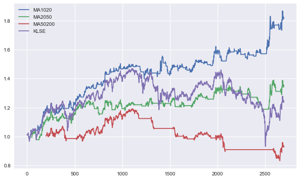

+----------+-------+----------+--------------+
| Strategy |  CAGR | Win Rate | Max Drawdown |
+----------+-------+----------+--------------+
|  MA1020  |  6.44 |  50.77   |     8.52     |
|  MA2050  |  3.14 |  30.77   |    12.15     |
| MA50200  | -0.89 |  28.57   |    30.08     |
+----------+-------+----------+--------------+

Thoughts

From the results, it seems like 10 and 20 moving average pair is the best
it consistently outperforms the benchmark.

The rest are disappointing,
longer term pairs are more likely to perform better in long bull runs index like SP500.

If you know coding,
you can try this out on other stocks that you like by getting csv data from Yahoo Finance.

This isn’t any trading advice and the studies and analysis done were for educational and sharing purposes only