用数据告诉你”布林线”在马股的有效性

布林线

布林线算是个常见的技术指标，
它的背后的数学相当优美

先用平均线当中线，
再用标准差 (standard deviation) 来计算上轨线与下轨线。

有点像标准正态分布 (normal distribution)。
背后的数学这里就不解释了

网上多的很，加上也没几个人想看。
大家关心的还是这个策略到底可不可以赚钱，

这篇文章我们来探讨这个策略在马股KLSE指数的表现如何。

数据读取

我从Yahoo Finance上下载了KLSE指数的历史数据，

要分析数据得先读取这个csv文件。

import pandas as pd

KLSE = pd.read_csv('KLSE.csv')
KLSE = KLSE.replace(',','', regex=True)
KLSE['Open'] = KLSE['Open'].astype(float)
KLSE['Close'] = KLSE['Close'].astype(float)
KLSE['Change'] = (KLSE['Close'] - KLSE['Close'].shift(1))/KLSE['Open'] + 1

KLSE.head()

	Date	Open	High	Low	Close	Adj Close	Volume	Change
0	4-Jan-10	1272.31	1275.75	1272.25	1275.75	1275.75	56508200	NaN
1	5-Jan-10	1278.26	1290.55	1278.26	1288.24	1288.24	136646600	1.009771
2	6-Jan-10	1288.86	1296.44	1288.02	1293.17	1293.17	117740300	1.003825
3	7-Jan-10	1293.69	1299.70	1290.36	1291.42	1291.42	115024400	0.998647
4	8-Jan-10	1294.93	1295.51	1290.86	1292.98	1292.98	74587200	1.001205

策略规则

这个策略的规则很简单，

要注意的是我们只Long，不Short，

毕竟在马来西亚卖空还是没那么容易的。

具体规则：

1. 收市价升破上轨线时，买入
2. 收市价跌破下轨线时，卖出Position
3. 收市价在上轨线和下轨线之内波动，不做任何买卖
4. 不考虑交易成本

def simulate(df,n):
    
    import talib
    
    df['UpperBand'], df['MiddleBand'],df['LowerBand'] = talib.BBANDS(df['Close'], timeperiod=n, nbdevup=2, nbdevdn=2, matype=0)
    
    df.dropna(inplace = True)

    gold_cross = df[df['Close'] > df['UpperBand']].index
    df.loc[gold_cross,'Cross'] = 1

    gold_cross = df[df['Close'] < df['LowerBand']].index
    df.loc[gold_cross,'Cross'] = 0
    
    df['Cross'].ffill(inplace=True)

    df['Buy'] = df['Cross'].diff()

    df['Return'] = df['Cross']*df['Change']

    def norm(x):
        if x == 0:
            return 1
        else:
            return x

    df['Return'] = df['Return'].apply(lambda x: norm(x))
    df['Nav'] = (df['Return']).cumprod()
    
    df.dropna(inplace=True)

    price_in = df.loc[df['Buy'] == 1,'Close'].values
    price_out = df.loc[df['Buy'] == -1,'Close'].values

    # divide by 252 because generally a year has 252 trading days
    num_periods = df.shape[0]/252
    rety = ((df['Nav'].iloc[-1] / df['Nav'].iloc[0]) ** (1 / (num_periods - 1)) - 1)*100.0

    if len(price_out) > len(price_in):
        price_out = price_out[:len(price_in)]
    
    if len(price_in) > len(price_out):
        price_in = price_in[:len(price_out)]
        
    VictoryRatio = ((price_out - price_in)>0).mean()*100.0
    DD = 1 - df['Nav']/df['Nav'].cummax()
    MDD = max(DD)*100.0

    return df, round(rety, 2), round(VictoryRatio, 2), round(MDD,2)

策略工作原理

这要解释也不容易，

还是上图吧！

绿箭头代表收市价升破上轨线，买入
红箭头代表收市价跌破下轨线，卖出 Position

Demo,_,_,_ = simulate(KLSE.copy(),20)

import matplotlib.pyplot as plt
plt.style.use('seaborn')

# Take a portion of the dataset to visualize, 
# Otherwise the plot will be too small
Demo = Demo[500:1000]

ax = Demo['UpperBand'].plot(figsize=(10, 6),alpha=0.7)
Demo['Close'].plot(ax=ax,color='navy')
Demo['LowerBand'].plot(ax=ax,alpha=0.7)


# Buy signal
for p in Demo[Demo['Buy'] == 1].index:
    ax.plot(p,Demo['Close'][p],marker='^',color='green',markersize=15)

# Sell signal
for p in Demo[Demo['Buy'] == -1].index:
    ax.plot(p,Demo['Close'][p],marker='v',color='red',markersize=15)

plt.show()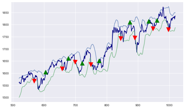

策略表现

我们测试3个设置，
分别是

1. 10天 (短期交易)
2. 20天 (中期交易)
3. 50天 (长期交易)

BBandShort,cagrShort,vrShort,mddShort = simulate(KLSE.copy(),10)
BBandMed,cagrMed,vrMed,mddMed = simulate(KLSE.copy(),20)
BBandLong,cagrLong,vrLong,mddLong = simulate(KLSE.copy(),50)


KLSE['KLSE'] = (KLSE['Change']).cumprod()


ax = BBandShort.plot(x='Date',y='Nav',figsize=(10, 6))
BBandMed['Nav'].plot(ax=ax)
BBandLong['Nav'].plot(ax=ax)
KLSE['KLSE'].plot(ax=ax)
ax.legend(['n= 10','n = 20','n = 50','KLSE (benchmark)']);
ax.set_title('Growth of RM1 Invested')
plt.show()


from prettytable import PrettyTable

t = PrettyTable(['Strategy', 'CAGR', 'Win Rate', 'Max Drawdown'])
t.add_row(['布林线 (10)', cagrShort,vrShort,mddShort])
t.add_row(['布林线 (20)', cagrMed,vrMed,mddMed])
t.add_row(['布林线 (50)', cagrLong,vrLong,mddLong])

print(t)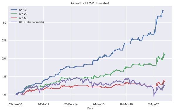

+-------------+-------+----------+--------------+
|   Strategy  |  CAGR | Win Rate | Max Drawdown |
+-------------+-------+----------+--------------+
| 布林线 (10) | 13.19 |   50.0   |     5.57     |
| 布林线 (20) |  7.94 |  46.88   |     5.57     |
| 布林线 (50) |  3.3  |  35.71   |     7.91     |
+-------------+-------+----------+--------------+

结论

从数据来看，胜率有点低，最高也只是50%
可是它看起来可以让交易者避免大规模下跌，参与升势。

而且大部分也都跑赢KLSE指数。
较长期的设置的表现较差强人意，

看起来布林线应该适合短期交易而已。

想要自己测试的读者可以从Yahoo Finance下载想要的个股数据来分析看看。

纯属分享，无买卖建议